
Siegfried Hörmann has been Professor of Applied Statistics at the Institute of Statistics of TU Graz since October 2017. Before this, he held professorships in the USA and Belgium.
The field of statistics has seen a big upsurge due to such new challenges. My research is devoted to some of these challenges.
Over the past decades storing and collecting data electronically has steadily become easier and cheaper. As a consequence, for many everyday life processes or scientific experiments nearly continuous data records exist. For example, on some engine test benches hundreds of variables can be collected and it is not uncommon to have for certain parameters of interest several measurement points per second. Similar examples can be given in environmental sciences (pollution levels), geophysics (strength of magnetic fields), medicine (fMRI images) or econometrics (tick-data), to just name a few. To benefit from increasing information, scientists need appropriate statistical tools which can help in finding the most important characteristics in such a big data context. Functional data analysis (FDA) is one of the emerging statistical disciplines which aims to extract relevant information from complex, intrinsically high¬dimensional data objects. It is targeted for data samples where each underlying sampling point is a curve or some other process defined on a continuum, such as a grey level image or surface temperatures, etc. (Figure 1).
 Statistics comes into play since we have replicates of the same experiment (measuring growth curves of individuals 1, 2, 3, ... and pollution levels on day one 1, 2, 3, ...). It is usually not particularly interesting if there was a peak PM10 load on a certain day at a certain time, but we may be very interested if peaks arise in a systematic way throughout a period of time. This will allow us to draw better conclusions regarding the polluters or to give better forecasts regarding the growth of a child. In both examples, there is variation and uncertainty between replicates due to very complex physical and biological processes, such as the nutrition regime and genetic endowments in the growth curves example. When a system becomes too complex to model all of its aspects, probabilistic and statistical tools enter the stage.

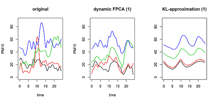 This approach, based on a so-called frequency domain analysis, not only allows for a better interpretation of the data, but is also useful in many problems of statistical inference. For the purposes of illustration, we show a 1¬dimenional approximation of four consecutive PM10 curves by means of the usual KL-expansion and dynamic functional PCA (Figure 4).
Kontakt
Siegfried HÖRMANN
Univ.-Prof. Mag.rer.nat. Dr.rer.nat.
Institute of Statistics
Kopernikusgasse 24/III
8010 Graz
Phone: +43 316 873 6476
<link int-link-mail window for sending>shoermann@tugraz.at
Growth curves and PM10
To clarify ideas, let us look at two simple FDA examples. In the first, we consider growth curves of 10 children at the age of 0¬18 years and in the second, we look at daily PM10 pollution level curves in Graz (Figure 2). In each curve we can check for many abstract features that may have practical or scientific relevance: e.g. the average level, the maximum, a potential trend or the position and number of peaks are important features in an environmental study on PM10 levels.Change in global surface temperature relative to 1951–1980.
Ten growth curves (left panel) and ten diurnal PM10 levels (right panel).
Tackling high dimension
In mathematical terms the curves that we investigate are realizations of a stochastic process. The fact that these random curves contain many features means that they constitute intrinsically high (in theory infinite) dimensional mathematical objects. From a practical as well as from a theoretical point of view, one is interested to reduce the dimensionality of the problem and to retain for a further analysis only those features in our observations which best describe the curves. A key statistical tool to tackle the dimensionality of functional data is the so-called functional principal component analysis. Functional principal components are orthogonal basis functions and as such we can use them to represent our functional observations as a superposition of these curves. This representation is called Karhunen-Loève (KL) expansion and its theoretical foundations date back to the early 20th century. Back then this approach was numerically unfeasible and hence it was not targeted for statistical applications. By expanding along a small number of basis-functions we obtain a low dimensional representation of the curve. The reader familiar with Fourier series may compare this to the Fourier expansion, where a curve is represented as a superposition of sinusoidal functions. The advantage of functional principal components is that, in some sense, they optimally adapt to the data. In Figure 3 we illustrate the approximation of a PM10 curve with 3 principal components and 5 and 25 Fourier basis functions, respectively.PM10 curve (upper left) and approximation with 3 principal components (upper right). Lower figures show the approximation by 5 (left) and 25 (right) Fourier basis functions.
Incorporating serial correlation
When looking at the PM10 and growth curve data, we observe several fundamental differences. For example, in contrast to PM10 data, the growth curves are monotone and smooth. Another important difference is that the growth data are statistically independent – there is no reason why the growth curve of one child should impact the growth curve of another child. This, however, is no longer true for the PM10 data. Not surprisingly, there is strong correlation between the PM10 loads on consecutive days. This problem is very common in FDA. It is related to the fact that many functional data are sampled sequentially in time (e.g. when data are obtained by segmenting a continuous process into natural units, such as daily data) which then often yields dependences. In one of my recent research projects I showed with my collaborators that the dependence between functional data can be used in order to obtain much more efficient dimension reduction than with common functional PCA. Our method is called dynamic functional principal component analysis.Four PM10 curves (left) and approximation with one dynamic principal component (middle) as well as one ordinary principal component (right).
Univ.-Prof. Mag.rer.nat. Dr.rer.nat.
Institute of Statistics
Kopernikusgasse 24/III
8010 Graz
Phone: +43 316 873 6476
<link int-link-mail window for sending>shoermann@tugraz.at